From zero to a useful query.

Open a file

Use it when you want to replace the current session and work with one main source. It supports Parquet, CSV/TSV, Excel, JSON/NDJSON, Arrow/Feather and R data.

1. Choose Open file or press Ctrl+O.
2. Pick the file; OliMat registers it as the data table.
3. The first page appears in Data & SQL and every other module is prepared with its schema.

Open a folder or dataset

Scans a folder and creates one table per supported file. Files can be CSV and Parquet with different structures; they are not concatenated automatically.

folder/
├─ catches.parquet  → table catches
├─ species.csv      → table species
└─ ports.xlsx       → table ports

It is the right option when the folder represents a whole project. If it contains partitions of the same dataset, check names and structure before deciding whether to query them together.

Add a file as a table

Keeps the current workspace and adds a new source. In the left tree you can expand columns, search, copy names and generate a SELECT.

SELECT c.date, s.name, c.catch_kg
FROM catches c
LEFT JOIN species s
  ON c.species_id = s.species_id;

Learn JOIN step by step

Save and reopen a .pvpw workspace

A portable project stores Parquet snapshots of the open tables together with the query, active table, favorites, history and dictionary. You can continue on another PC even if the original files or the Oracle connection are no longer available.

1. After preparing your tables, choose File ▸ Save workspace or press Ctrl+S.
2. Save the .pvpw file; wait for the operation to finish before copying it.
3. Open it with File ▸ Open workspace or, since version 4.49, by double-clicking if you installed the association.

Excel with several sheets, titles and merged headers

When you open a workbook with more than one sheet, a picker appears with each sheet's name and size (chart-only sheets are excluded automatically). Every sheet you tick becomes its own table — and you can JOIN across sheets.

1. Open the .xlsx; tick the sheets you care about.
2. If a sheet has a title or loose rows above the table, set the Range (e.g. A5:H200) starting at the header row.
3. Accept: each sheet becomes an independent workspace table.

Data & SQL

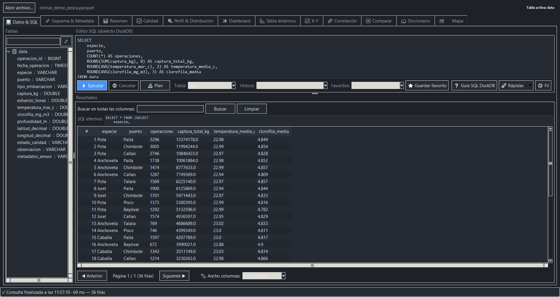
Real query over 85,000 synthetic rows. The grid renders only the visible page.

• Editor: write DuckDB SQL and run with Ctrl+Enter.
• Effective SQL: shows how filters and sorting modify the query.
• Grid: sort, filter, search and paginate without drawing millions of rows.
• Quick queries: build SELECT, COUNT, summary, top values, nulls or samples.
• Plan: use EXPLAIN ANALYZE to understand heavy queries.

Filter without writing SQL

The 🧩 Visual filter button (in Data & SQL) builds the query for you and shows it: the fastest way to learn by seeing.

1. Press 🧩 Visual filter and choose column, operator and value. The value dropdown loads that column's most frequent values.
2. Add more conditions and decide whether all (AND) or any (OR) must match.
3. Watch the generated SQL at the bottom and press ▶ Apply filter.

Review table structure and summary

1. Open Schema and confirm every name and type matches expectations.
2. Use tree search to locate columns; right-click to copy a name, generate SELECT, rename or activate a table.
3. Open Statistics to review rows, columns, cardinality and numeric summaries.
4. If a type does not represent the content, return to Data & SQL and create a safe conversion with TRY_CAST.

Investigate data-quality warnings

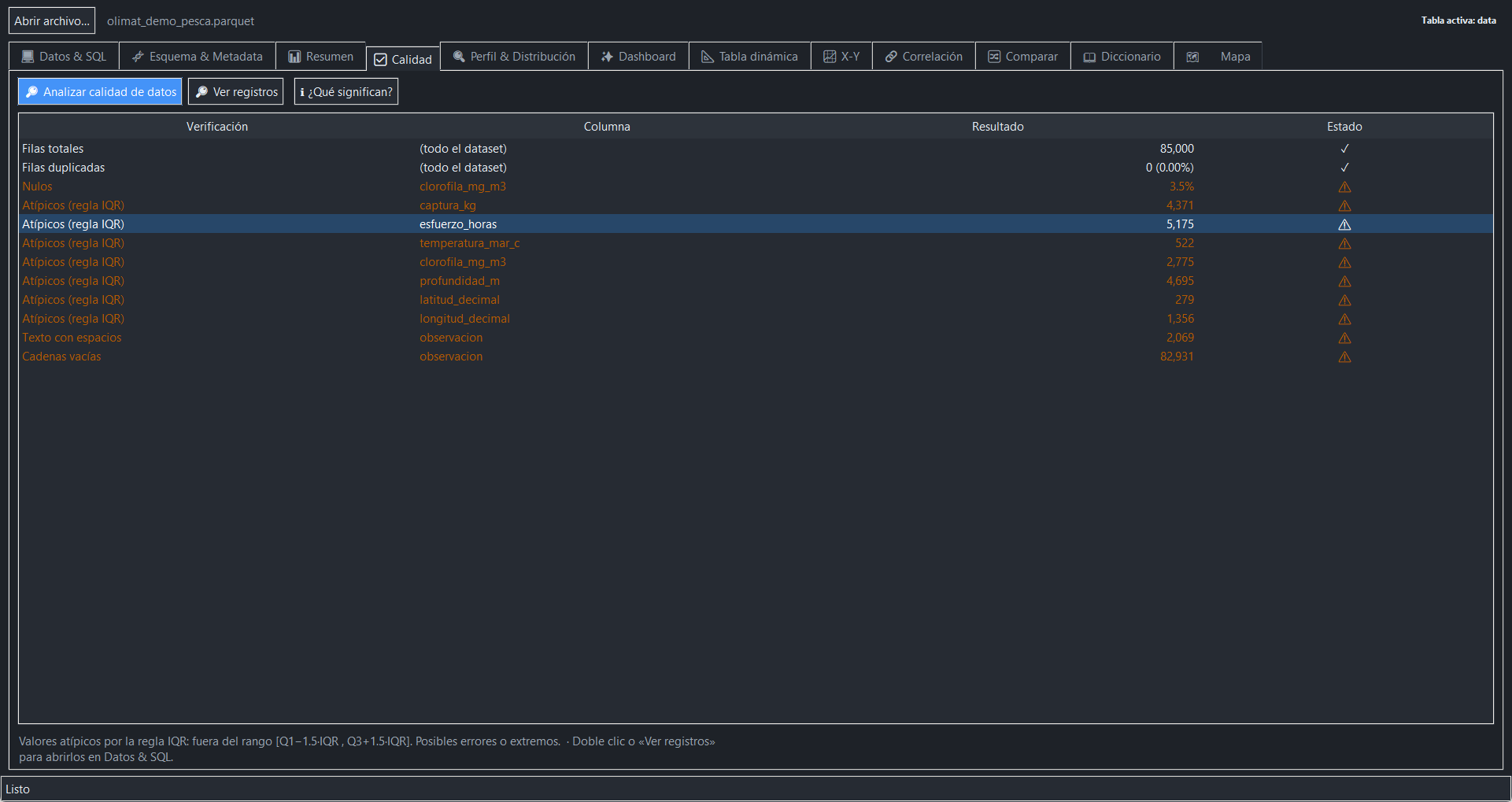
Select a warning to read its meaning and open the affected records.

1. Open Quality and run the analysis on the active table.
2. Select a warning for nulls, duplicates, empties, whitespace, mixed types or outliers.
3. Read its explanation and open affected rows in Data & SQL.
4. Use domain knowledge to decide whether it is an error or a valid value.

Quality rules that are remembered

In the Quality tab, "Saved quality rules" section: define your own validations once and revalidate whenever a new version of the file arrives.

1. Press + Rule and choose column and type: no nulls, unique values, numeric range, pattern (regex), allowed values list or maximum length.
2. Press ▶ Validate rules: each rule shows ✓ or the number and percentage of violations.
3. Double-click a failing rule to open the affected rows in Data & SQL, ready to fix or export.

Full profile in one click

In the Profile tab, the 📋 Full profile (HTML) button generates a technical sheet of every column: type, % nulls, uniques, min/max, mean, quartiles and most frequent values.

1. Press the button and choose where to save the report.
2. It opens automatically in your browser; it is a single self-contained HTML file.
3. Attach it to an email, a repository or a records file: it looks good in light and dark and needs no internet.

Get an automatic first reading

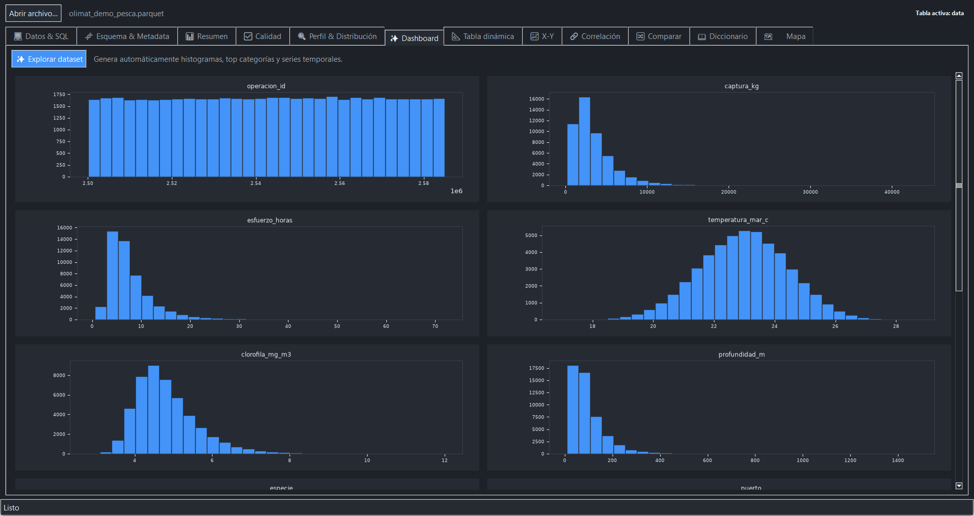
Content adapts to the active table's column types.

1. Select a table in the tree and open Dashboard.
2. Review numeric distributions, top categories and available time series.
3. Use a finding to choose which column to profile or which filter to apply.
4. Formalize important analysis in Data & SQL so it can be repeated.

Build a pivot table

1. Open Pivot and choose a field for Rows.
2. Optionally choose Columns to cross categories or periods.
3. Select the Measure and aggregation: sum, average, count, minimum or maximum.
4. Run it, review totals and export if it belongs in the deliverable.

Visualize a relationship or distribution

1. Open X-Y Chart and choose axis variables.
2. Select an available chart type and, when relevant, a grouping or color column.
3. Adjust sample size to balance detail and speed.
4. Interpret the pattern alongside both column profiles; do not mistake association for causation.

Calculate Pearson or Spearman

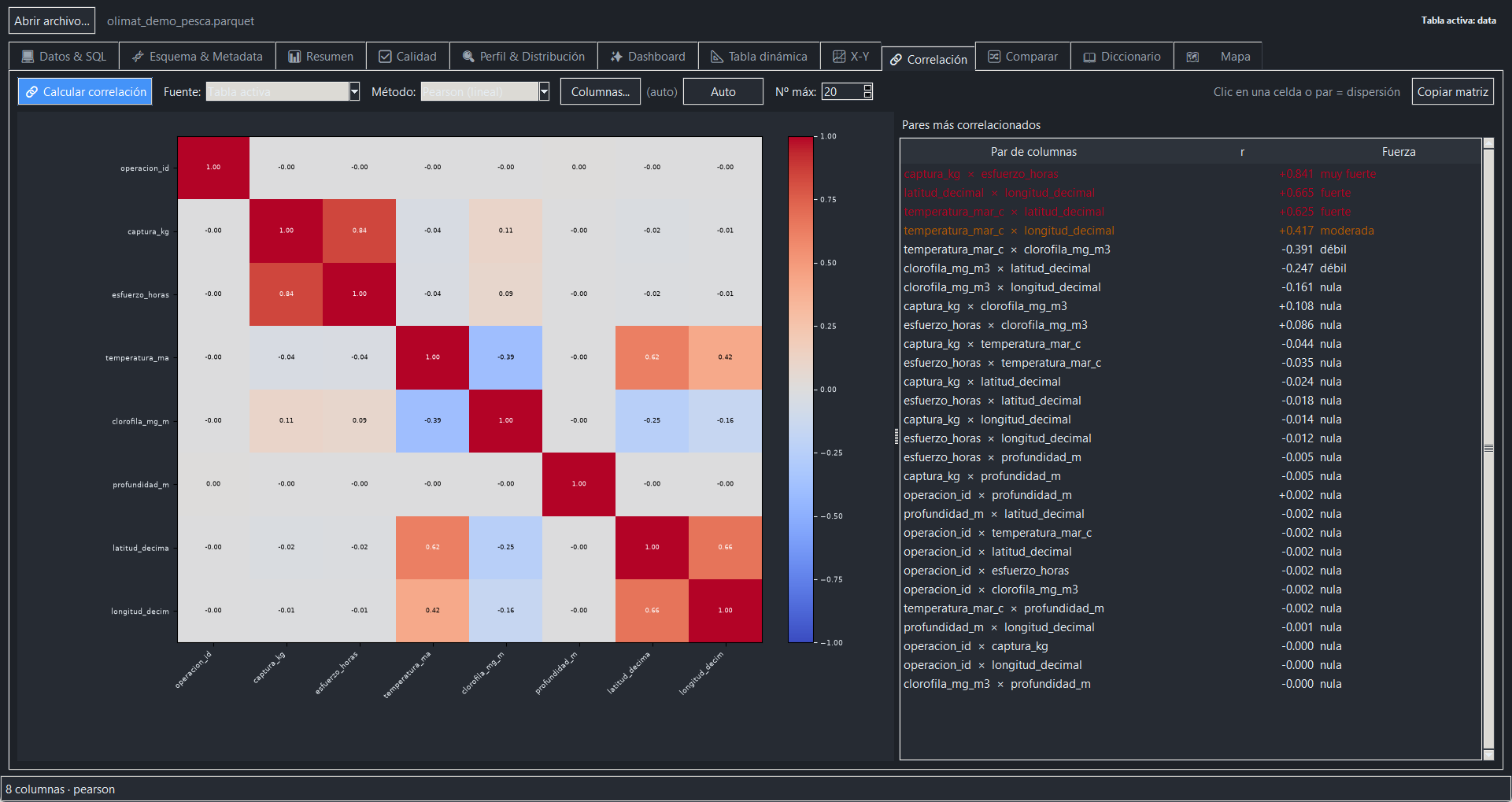
The matrix summarizes strength and direction; pair detail shows the relationship's shape.

1. Open Correlation and select relevant numeric columns.
2. Use Pearson for linear relationships or Spearman for monotonic rank relationships.
3. Run the calculation and sort pairs by absolute value.
4. Open a pair as scatter and inspect outliers, groups or nonlinear shapes.

Compare two tables or deliveries

1. Add both sources to the workspace and give them unambiguous names.
2. In Compare, select the baseline and candidate tables.
3. Run it and review differences in columns, types, rows and nulls.
4. To locate specific records, run a JOIN or ANTI JOIN by key in Data & SQL.

Learn JOIN and ANTI JOIN

Document columns and preserve context

1. Open Dictionary and select the table.
2. Complete description, unit, value domain or notes for each column.
3. Export the dictionary when it must be shared outside OliMat.
4. Save the .pvpw workspace to retain the dictionary with tables and queries.

Create a map and filter an area

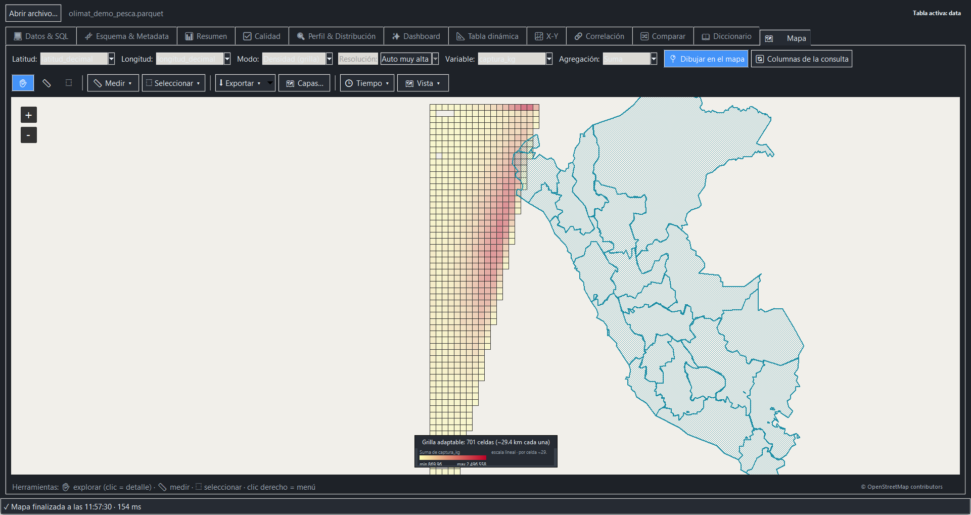
Grid weighted by catch and departments loaded from a Shapefile.

1. Choose the latitude and longitude columns; they may arrive as convertible text.
2. Select Points or Density (grid).
3. Optionally choose a numeric variable and an aggregation.
4. In Time, pick a date column and adjust start/end.
5. Use Select for box, lasso, circle or polygon and send the filter to the results.
6. Use Measure for distance, radius, perimeter or area.

The grid can adapt to the screen or use an approximate size in kilometres. More resolution creates more cells; increase gradually to keep the map readable.

Use the map without internet and export it as PNG

Every map area you visit is stored automatically on your machine and reused offline. There is nothing to download in advance: OpenStreetMap's policy forbids bulk area downloads, and what it does allow (and require) is exactly this browsing cache.

1. While online, browse your working area at the zoom levels you will need.
2. Press 📴 Offline to see how much your local cache holds.
3. Done: those areas will work without a connection in your next sessions.

To take the map into a report: Export → 🖼 Export image (PNG). The image includes the density legend, a scale bar and the provider attribution: ready to paste into Word or a presentation.

Open RDS or RData without having R

An .rds can contain one table or a list with dozens of them. The app catalogs them without loading and converts only what you choose.

1. Open the .rds/.RData file like any other.
2. If it holds several tables, the catalog appears with each one's name, rows and columns: tick the ones you need.
3. Each chosen table is converted to cached Parquet and becomes available for SQL, the map, profiling and exports.

CSV files with accents that other tools reject

CSV exported by Excel, Oracle or legacy systems often arrives as Latin-1/Windows-1252 (or UTF-16 from SQL Server/PowerShell) and fails in viewers that expect UTF-8. Here there is nothing to configure:

1. Open the CSV normally.
2. If it is not UTF-8, the app detects the encoding from the bytes and retries by itself.
3. Ñ, accents and symbols like € come out correct, and the view stays configured for the rest of the session.

Nested JSON without unexpected multiplication

A trip with one activity, one species, 20 biometric and 15 biological records stays as one row with nested arrays. The cell viewer lets you expand each branch.

You only get 300 combinations if you explicitly take the product of both arrays. To keep relationships separate, flatten each array in its own query or table.

-- Flatten only biometrics
SELECT trip_id, activity.unnest AS activity,
       biometric.unnest AS biometric
FROM data,
UNNEST(sp_activity) AS activity,
UNNEST(activity.sp_species) AS species,
UNNEST(species.sp_biometric) AS biometric;

Import a query or export a table

1. Choose Import from Oracle and enter host, port, service and user. The password is used for the session and is not stored.
2. Test the connection and run a query limited to the required columns and rows.
3. Name the imported table; it then behaves like any local workspace table.
4. To send a result back, choose Export to Oracle, review destination and permissions, then confirm.

Export results

Exports start from the effective query, not just the visible page. Choose Parquet to preserve types and performance, Excel for manual exchange, CSV for compatibility, GeoJSON for GIS, Arrow/Feather for data science, or SQLite for a portable database. You can also generate SQL INSERT statements or send the result to Oracle.

Errors, cancellation and performance

• An invalid query shows the DuckDB message — with a plain-language explanation for the common ones — and keeps the app open.
• TRY_CAST prevents a single bad value from breaking numeric or date conversions.
• Pagination protects the interface; avoid exporting millions of INSERTs when Parquet or CSV serve better.
• In large JOINs, select only the needed columns and filter early when possible.